Parallel BVH Construction on a CPU
Brian Fischer(bfischer) and Ian Huang(ijhuang)
Summary
We implemented three parallel BVH construction algorithms on a CPU using Approximate Agglomerative Clustering(AAC) and compared its build time to each other and to a Surface Area Heuristic(SAH) implementation. In addition, we also compared performance in ray tracing between the AAC builds and SAH build. We tested our algorithms on a consumer computer with a quad core lntel Core i7-3720QM CPU at 2.60GHz. Our AAC algorithm uses a divide and conquer technique, which is a natural fit for Cilk+. Our contributions are an extension to Matt Pharr and Greg Humphreys's PBRT ray tracer.
Background
Ray tracing is used for rendering 3D scenes. In forward ray tracing, photons from a light source are traced through the scene. In backward ray tracing, rays are shot from the camera and are traced through the scene. Rays shot in this manner correspond to pixels in the rendered image.
 Figure 1: Backward Ray Tracing
One of the main steps involved during Ray Tracing is intersection tests with primitives in the scene when casting rays. However, there is no need to check for intersections among all primitives in the scene because the probability of a ray hitting a given primitive is very low. Thus, to reduce the number of primitives we need to check a ray against, we use spatial data structures.
Bounding Volume Hierarchy(BVH)
A Bounding Volume Hierarchy(BVH) is a binary tree that stores primitives in the scene. Each node in the tree represents a bounding volume. Bounding volumes at the top of the tree represent larger areas of the scene, while nodes at the bottom of the tree represent smaller areas. When casting rays, we traverse the tree, checking if we hit the bounding volume of the node. If we do, we traverse down to both left and right children of the node and run the same test.
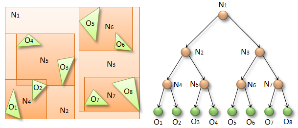 Figure 2: Bounding Volume Hierarchy
BVH construction can be done using a divide and conquer process and is naturally parallel. Top-down and bottom-up methods of construction exist. Leaf nodes can consist of one primitive or multiple depending on whether or not it is cheaper to check for intersections among multiple primitives or to search a deeper tree.
Morton Codes(Z-Order Curve)
Morton Codes are used to map primitives from multidimensional space to 1D space while preserving locality. Triangles can be mapped to Morton Codes using their centroid. The Morton Code for a 3 Dimensional point interleaves the x, y, and z coordinates of the point in a number. If we store a Morton Code in a long, 10 bits are used for each of the x, y, and z coordinates. The remaining 2 bits can be used as flags.
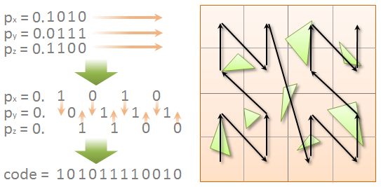 Figure 3: Morton Codes
For BVH construction, morton codes are used to partition elements on a particular axis. Partitioning in this manner works for approximate clustering since Morton Codes preserve locality.
Agglomerative Clustering
Agglomerative Clustering is an algorithm for clustering objects based on distance. However to do so, it has to check all clusters to find the closest neighbor. This is computationally expensive as it requires n^2 comparisons when combining clusters, and has total n^3.
Approximate Agglomerative Clustering(AAC) limits the candidates considered when searching for the nearest neighbor. Rather than comparing all objects for the closest neighbor, AAC groups primitives based on sorted Morton Codes.
AAC consists of three main phases. In the first phase, primitives’ Morton Codes are computed and then sorted. Sorting the Morton Codes allows us to easily partition the primitives based on bits of the Morton Codes. For given bit position i, we can just do a binary search of the sorted morton codes to see where bit i changes from 0 to 1. This also rotates partitioning the primitives along the x, y, and z axes.
In the second phase, the “downward” phase, the sorted primitives are partitioned based on each digit of the Morton code(0 or 1), starting from the most significant bit of the code. Partitioning continues until we reach a threshold. Once few enough primitives remain, we can begin clustering the primitives by first creating a cluster for each primitive. The threshold at which we begin clustering can be set a higher number to improve the resulting BVHs quality, or set to a lower number to improve the construction time.
In the third phase, the “upward” phase, the clusters are combined using a brute force agglomerative clustering method. Using the brute force method to cluster here is cheap since we are running it on a small number of clusters. The tree is formed by grouping the closest clusters as children of a BVH node. At any step, we keep combining clusters until the desired number of clusters remain and then return. The remaining clusters will be combined with the clusters returned from other instances of the third component. This bottom up construction continues until only one cluster remains(the root of the BVH).
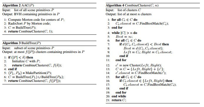 Figure 4: Approximate Agglomerative Clustering Pseudocode
Approach
We started with the Physically Based Rendering Raytracer(pbrt-v2) as a basis for our project. PBRT already contains a BVH library that implements several construction methods including partitioning by the node’s midpoint, partitioning into two equal sized sets of primitives, and partitioning using Surface Area Heuristic. The Surface Area Heuristic(SAH) method performs the best out of the three in terms of BVH quality, and is the method we decided to compare against. Construction methods were evaluated in two ways. The first was the time it took for BVH construction. The second was the performance of the PBRT Raytracer when using the BVH. A better quality BVH will have lower intersection test costs and lower number of node traversals than that of poorer quality. All AAC implementations use a data parallel computation model.
Brute Force AAC
In our first iteration of AAC, we implemented a brute force version. In this version, FindBestMatch(in algorithm 4) uses an n^2 approach to finding the closest node to each node by calculating the distance between all nodes. However, this is inefficient because each iteration of FindBestMatch will calculate the distance d(c1, c2). This requires loading two cluster bounding boxes from memory and then calculating an aggregate bounding box and its surface area. However, this version is nice because it has an embarrassingly parallel structure. Thus BuildTree(algorithm 3) is very easy to implement and we also have fine grain parallel tasks for even workload distribution among cores.
We then implemented another version which stored distances in a two dimensional array. Here we only need to use half of the array because distance[i,j] is the same as distance[j,i]. Figure 5 shows how the distance matrix is filled. First we get the results of Buildtree(left). We then use the size to figure out how much of the matrix was used for the left. We then do BuildTree(right), which will write to the triangle on the diagonal immediately after the left. Then we merge the data by filling in the missing data: the distances between the clusters in the left and the clusters in the right. Here we see that we have created a dependency between the two calls to BuildTree. We must know the size of the left tree before calling BuildTree on the right. If we did not and just decided to give each call enough space, our data would be spread out and we would lose spatial locality. However, this method reduces memory movement and allows for reuse of computations. Thus we trade parallelism for better memory management.
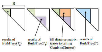 Figure 5: Data Reuse
We looked at two different approaches to parallelize the BVH construction with this new optimization.
Memoized AAC
The first approach spawns multiple subtasks in parallel. When the subtasks return, they are stored in a task tree. When all the subtasks return, we call a separate function to take the task tree and merge the results sequentially. Ideally, the merges near the top of the tree should be cheap, because we will have fewer clusters. In addition, we can spawn enough subtasks(about 8x the core count) to ensure we have enough parallelism for many cores.
Hybrid AAC
The second approach is a hybrid approach which uses a brute force method at the top nodes of the tree and a computation reuse method for the bottom nodes of the tree. Like the first approach, we first spawn multiple subtasks in parallel, however, as they return, we can combine the clusters in parallel by using the brute force method which recalculates distances between clusters. This way, we remove all dependencies at the top of the tree and thus gain more parallelism.
Other Optimizations
In addition to optimizing the building phase, we also optimized the sorting done beforehand. We implemented a parallel radix sort based off the block radix sort in the Parallel Benchmark Suite. This does not improve performance on scenes with lower number of triangles, but will improve the sorting time on scenes with larger number of triangles.
Results
We performed experiments on a quad core lntel Core i7-3720QM CPU at 2.60GHz. We tested performance on 3 scenes, Buddha, Yeah, Right, and Villa. BVH construction methods were evaluated in 2 ways. The first was the speed at which the trees were constructed. The second was the performance of the BVH when used by the PBRT Raytracer.
As a side note, BVHs must be constructed a certain way to be used by PBRT. In our case, we had to perform a depth first search on our BVH at the end of construction in order to be processed correctly by PBRT. This DFS is sequential is unable to be sped up. Thus we only profile the code we focused on, the parallelizable AAC construction code.
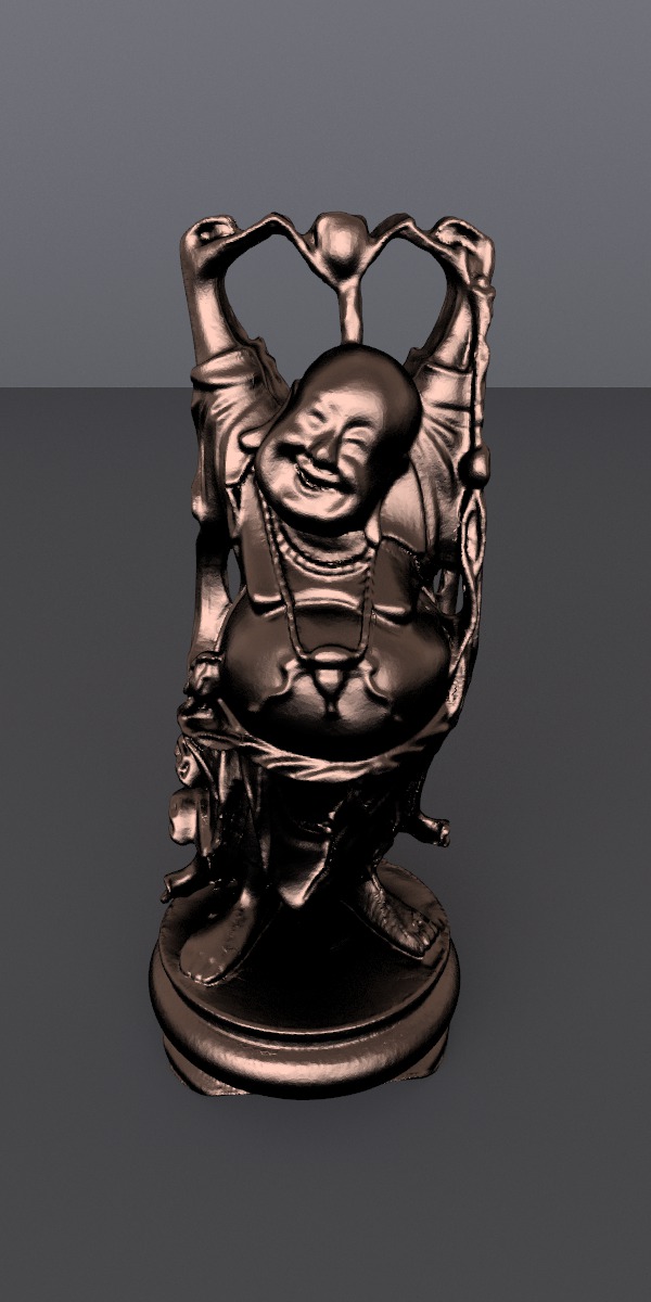
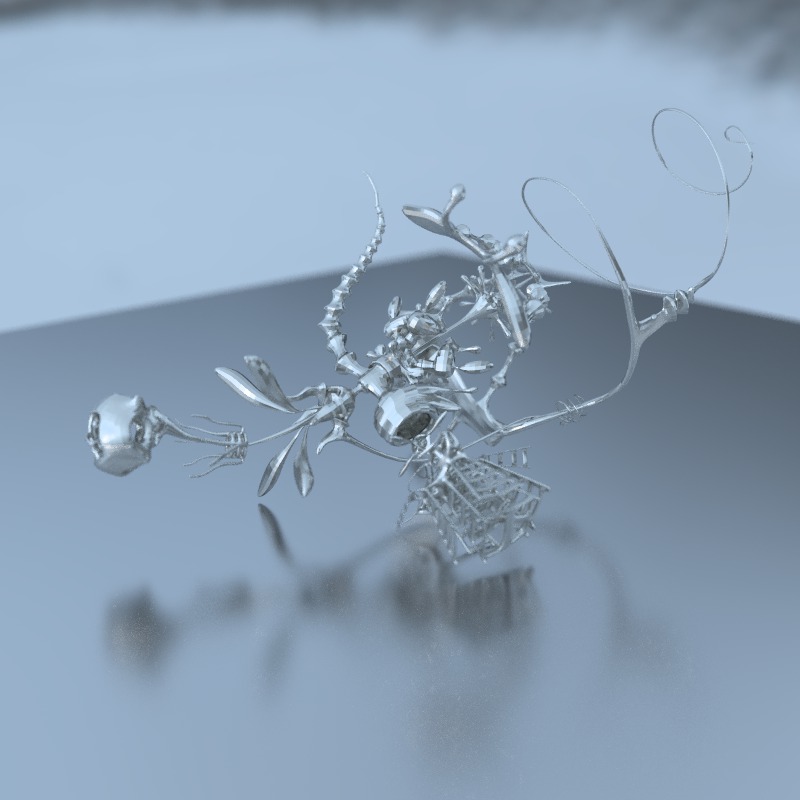 Figure 6: Buddha(1087720 Primitives) and Yeah, Right(188674 Primitives)
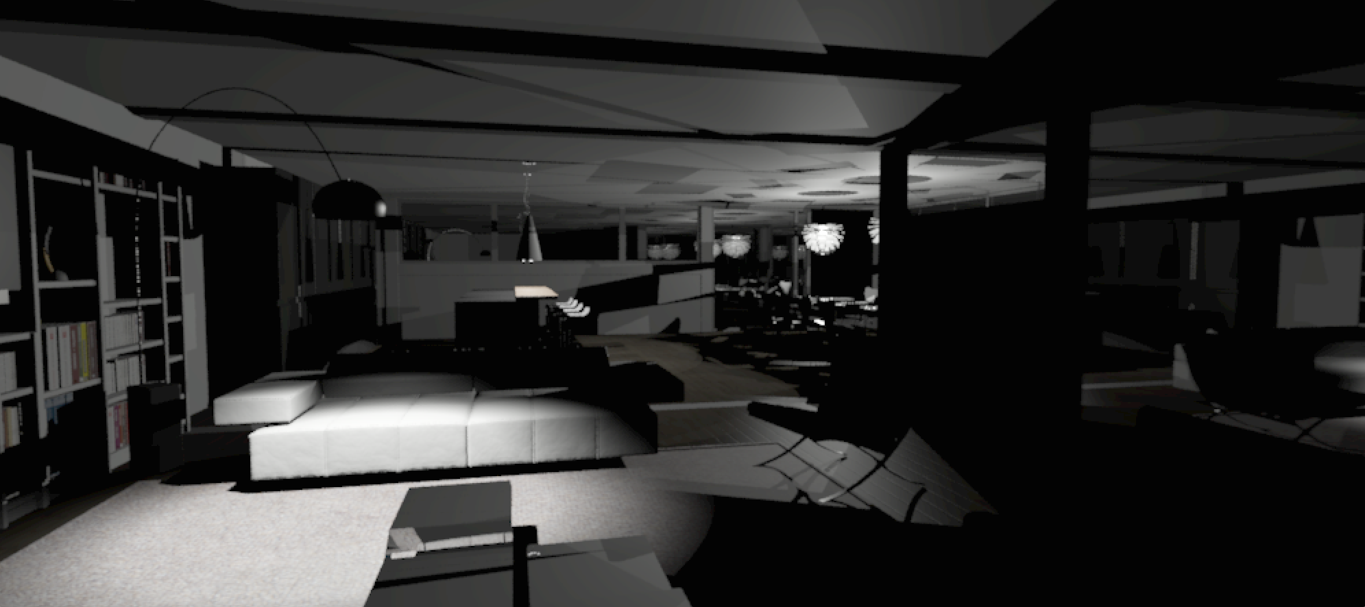 Figure 7: Villa(2547152 Primitives)
The three scenes varied in size. Buddha has 1.1 million primitives. Yeah, Right has 188.6k primitives. Villa has 2.5 million primitives. For all problem sizes, we achieve good speedups. Ray tracing generally uses many primitives, resulting in large problem sizes with lots of parallelism.
Construction Time and Speedup
We measured the construction time and speedup for BVH construction using various cilk workers and scenes.

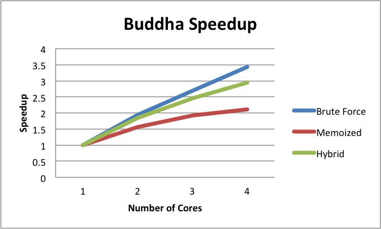 Figure 8: Buddha Construction Time and Speedup
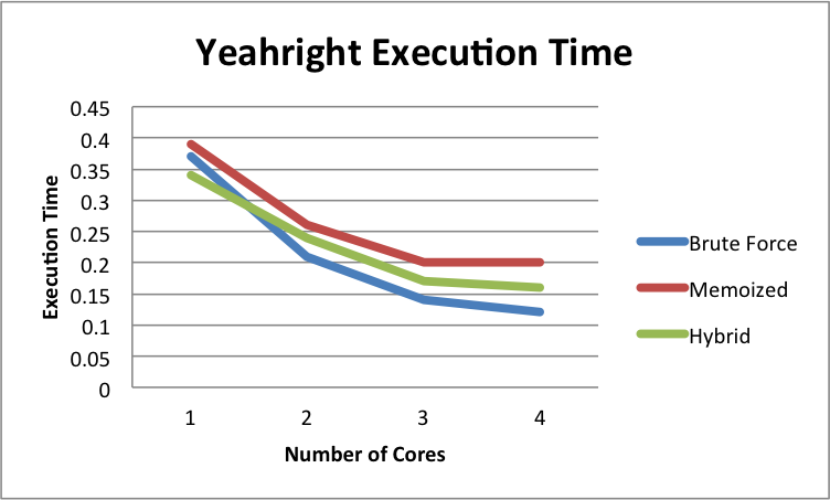
 Figure 9: Yeah, Right Construction Time and Speedup

 Figure 10: Villa Construction Time and Speedup
The graphs above show speedup for the parallelizable portions of our code. As we can see, we gain nearly linear speedup up to 4 cores for all algorithm.
Using the Brute Force method, we achieve nearly linear speedup on all three scenes. This is expected as Brute Force is the method with the most parallelism. It also has fine grain parallelism, since the base case consists of small problem sizes (< 20). Thus we can evenly distribute work across all cores. We would expect this trend to continue for higher core counts, and do not expect the program to be either compute or bandwidth bound.
The memoized method has less of a speedup compared to brute force. This is expected, because there is less parallelism here. There is a significant amount of time spent processing the results of the subtasks in serial as seen in Table 1 (up to ~30% on Yeah, Right). In addition, the granularity of parallel tasks is much larger. Since we spawn these subtasks high in the tree, we may have many subtasks with different problem sizes. This can cause an uneven distribution of work among processors. One way to remedy this is to create more subtasks by creating subtasks lower in the Divide and Conquer tree. However, by creating more subtasks, we have also created more subtasks to process in serial, and thus we will have a larger serial portion than before.
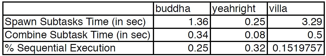 Table 1: Execution Time Breakdown for Memoized Construction on 1 core
The Hybrid method is somewhat of a compromise between the brute force and memoized methods. While we still have larger granularity sub tasks being executed in parallel, we no longer have a large portion of our building time running sequentially. Thus we have more parallelism, and we can also create subtasks lower in the Divide and Conquer tree. We see in our performance results that our hybrid approach takes a middle ground between our brute force and memoized methods.
We analyzed the execution time of specific regions of our algorithm using the Villa scene(Table 2). We executed our AAC algorithms on 1 core to observe what percentage of our code was sequential or unrelated to the divide and conquer algorithm. When constructing the BVH using the brute force method, we found that sorting the Morton codes takes ~2% of the overall execution time and performing the in order traversal of the BVH for PBRT takes ~18% of the overall execution time. In our memoized and hybrid version, we found that allocating memory for the tables also took a nontrivial amount of time. The rest of the time is spent constructing the BVH. We found that when testing other methods of BVH construction, specifically surface area heuristic, these phases take roughly the same amount of time and percentage of computation.
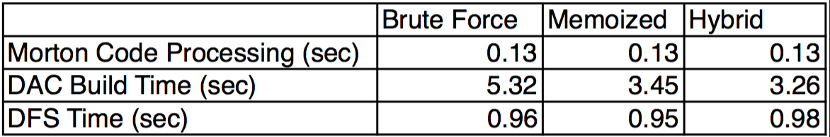 Table 2: Breakdown of Timings Spent in Each Phase of AAC on 1 core
We compared rendering times for SAH versus our three versions of AAC for each scene. In each scene, both methods had roughly the same rendering time. In [1], we see that AAC should generally yield higher quality BVHs and thus have faster rendering times. This is due to the BVH flattening technique that is made possible by AAC (discussed as an optimization in [1]). However, our main focus was on BVH construction performance, and thus we decided not to implement this optimization and instead focus on construction optimizations.
In Table 3, we compare the construction times of SAH against our three AAC methods. Note that these AAC timings include Morton Code sorting as well as an in order DFS traversal to be consistent with the SAH method. As we can see, SAH is faster than all three methods when executing on a single core. While we did not extensively test this, we believe this is due to PBRT’s usage of its sequential memory allocator called Memory Arena. It allocates many blocks of data at a time, and manages the blocks by distributing them to processes and keeping counters on the blocks. However, PBRT’s Memory Arena is not thread safe and cannot be used in multi threaded code. Thus, we decided just use the standard C allocators. We also did not achieve the same timings as [1] but after speaking to the authors we decided it was out of the scope of this project as they implemented many difficult optimizations, some involving assembly hacking.
 Table 3: BVH Construction Results
Approximate Agglomerative Clustering is a highly parallelizable algorithm. There is enough parallelism available to make use of all the resources available on many core processors. While we chose to use a CPU, implementing AAC for GPUs is an interesting problem that we would like to look into in the future.
One issue we had was we were unable to profile our code on a 40 core machine we had access to. We were able to compile and run the code, but the machine provided results extremely inconsistent from the results in [1] and results on our quad core machine. We have looked into it, but cannot say exactly what causes this. We speculate that it could be due to the different environment and compiler. We also could not run on Latedays because the version of GCC did not support the cilk_for keyword and when attempting to compile with ICC, we would get compilation errors.
References
- Efficient BVH Construction via Approximate Agglomerative Clustering
- Fast BVH Construction on GPUs
- Thinking Parallel Part II: Tree Construction on the GPU
- PHARR, M., AND HUMPHREYS, G. 2010. Physically Based Rendering: From Theory to Implementation, 2nd edition. Morgan Kaufmann Publishers Inc., San Francisco, CA, USA.
Code
Github Repository
List of work by each student
Equal work was performed by both project members